pykp.metrics.

phase_transition#

pykp.metrics.phase_transition(num_items: int, samples: int = 100, outcome: str | tuple = ('solvability', 'time', 'cost'), solver: str = 'branch_and_bound', minizinc_solver: str = 'coinbc', resolution: tuple[int, int] = (41, 41), seed: int | None = None, path: str = None, weight_dist: str = 'uniform', value_dist: str = 'uniform', weight_dist_kwargs: dict | None = None, value_dist_kwargs: dict | None = None) → tuple[ndarray, ndarray]#

Compute the phase transition matrix for knapsack instances.

In computational problems, a phase transition refers to a phenomenon where the probability of finding a solution changes abruptly as some parameter crosses a critical threshold. This concept draws inspiration from physics, where phase transitions (e.g., water freezing) occur at critical thresholds. Such transitions have also been shown to arise in NP-complete problems, where the likelihood of finding a solution changes abruptly as a key parameter crosses a critical value.

For an \(i\) item knapsack instance with capacity \(C\) and target profit of \(T\), this phase transition manifests in terms of the relationship between the normalised capacity (c) and normalised profit (p) of an instance, [1] where

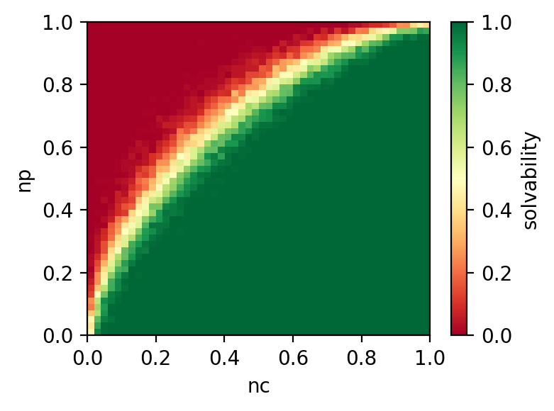
\[c = \frac{C}{\sum_{i=1}^{n} w_i} \quad \text{and} \quad p = \frac{T}{\sum_{i=1}^{n} v_i}.\]

The phase transition matrix is a 2D grid over c and p, where each cell represents the proportion of instances that are satisfiable at that point in the grid. The phase transition matrix can be used to identify regions of the (c, p) parameter space where the problem is more or less likely to be satisfiable. The proportion of satisfiable instances in each cell has been shown to be preditive of both human and algorithmic performance on knapsack problem instances.

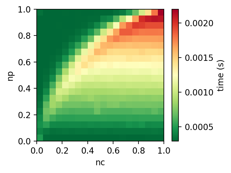
A similar phase transaction matrix can be computed for the average time taken to solve instances in each cell, or the number of propagations required to solve each instance.

Parameters:

num_itemsint: Number of items in each generated knapsack instance.
samplesint, optional: Number of instances to evaluate in each cell of the grid. Default is 100.
outcomestr | tuple, optional: The outcome to measure in each cell. One or more of “solvability” “time” or “cost”. If “solvability” is specified, the phase transition matrix represents the proprotion of instances that are satisfiable in each cell. If “time” is specified, the phase transition matrix represents the average time taken to solve instances in each cell. If “cost” is specified, the phase transition matrix represents the maximum cost (e.g. number of propagations) required to solve instances in each cell. Default is (“solvability”, “time”, “cost”).

Returns:

coordinate_matricestuple of np.ndarray: The coordinate matrices for normalised capacities and normalised profits. The first matrix corresponds to normalised capacities, and the second to normalised profits.
phase_transitionnp.ndarray: If outcome="solvability", a 2D matrix where each cell represents the proportion of instances that are satisfiable. If outcome="time", a 2D matrix where each cell represents the average time taken to solve instances. If outcome="both, a tuple containing both matrices.

Other Parameters:

solverstr, optional: Which solver to use for evaluating each instance. Default is “branch_and_bound”.
minizinc_solver: str, optional: If solver="minizinc", this argument specifies which minizinc solver to use. Default is “coinbc”.
resolution: tuple[int, int], optional: Resolution of the normalised capacity-normalised profit grid. The first element corresponds to the resolution of normalised profit, and the second to the resolution of normalised capacity. Defaults to (41, 41).
weight_diststr, optional: Name of the distribution to sample item weights from. Defaults to uniform distribution over the half-open interval [0.001, 1).
weight_dist_kwargsdict, optional: Additional keyword arguments to pass to the weight distribution function. Defaults to None.
value_diststr or tuple, optional: Name of the distribution to sample item values from. Defaults to uniform distribution over the half-open interval [0.001, 1).
value_dist_kwargsdict, optional: Additional keyword arguments to pass to the value distribution function. Defaults to None.
seedint | None, optional: Seed for sampling. Defaults to None.
path str, optional:: Path to save the phase transition to. Defaults to None.

Notes

The phase transition is typically applied with reference to the decision variant of the knapsack problem. To apply the phase transition to the optimisation variant, the target profit should be set to the optimal solution value of the instance. One can then compute the normalised profit based on the optimal solution, and observe where the instance lies in the phase transition matrix.

References

Examples

>>> from pykp.metrics import phase_transition
>>> grid, (solvability, time) = phase_transition(
>>>     num_items=12,
>>>     samples=1000,
>>>     outcome="both",
>>>     solver="branch_and_bound",
>>>     resolution = (20, 20),
>>> )
>>> grid[0].shape, grid[1].shape, solvability.shape, time.shape
((20, 20), (20, 20), (20, 20), (20, 20))

Visualise the phase transition matrices using matplotlib:

>>> import matplotlib.pyplot as plt
>>> fig, axes = plt.subplots(
...     nrows=1,
...     ncols=1,
...     dpi=200,
...     figsize=(4, 3),
...     tight_layout=True,
... )
>>> image = axes.imshow(
...     phase_transition,
...     cmap="RdYlGn",
...     interpolation="nearest",
...     aspect="auto",
...     extent=(0, 1, 0, 1),
... )
>>> axes.set(xlabel="nc", ylabel="np")
>>> cbar = fig.colorbar(image, ax=axes)
>>> cbar.ax.set_ylabel("solvability"
>>> plt.show()

>>> fig, axes = plt.subplots(
...     nrows=1,
...     ncols=1,
...     dpi=200,
...     figsize=(4, 3),
...     tight_layout=True,
... )
>>> image = axes.imshow(
...     phase_transition,
...     cmap="RdYlGn_r",
...     interpolation="nearest",
...     aspect="auto",
...     extent=(0, 1, 0, 1),
... )
>>> axes.set(xlabel="nc", ylabel="np")
>>> cbar = fig.colorbar(image, ax=axes)
>>> cbar.ax.set_ylabel("time"
>>> plt.show()

Optionally save results to file by specifying a path:

>>> phase_transition(
...     num_items=10, samples=50, resolution=(5, 5), path="output.csv"
... )